由kaggle房价模型得到stacking model方法

房价模型在kaggle房价预测问题中已经介绍过,具体不再赘述。

大致内容为:根据给定的数据的80个变量来预测未知数据(同样包含80个变量)来预测房价

首先导入需要的包

1
2
3
4
5
6
7
8
9
10
11
12
13
14
15
16
17
18
19
20
21
22
23
24
#import some necessary librairies

import numpy as np # linear algebra
import pandas as pd # data processing, CSV file I/O (e.g. pd.read_csv)
%matplotlib inline
import matplotlib.pyplot as plt # Matlab-style plotting
import seaborn as sns
color = sns.color_palette()
sns.set_style('darkgrid')
import warnings
def ignore_warn(*args, **kwargs):
pass
warnings.warn = ignore_warn #ignore annoying warning (from sklearn and seaborn)


from scipy import stats
from scipy.stats import norm, skew #for some statistics


pd.set_option('display.float_format', lambda x: '{:.3f}'.format(x)) #Limiting floats output to 3 decimal points


from subprocess import check_output
print(check_output(["ls", "../input"]).decode("utf8")) #check the files available in the directory

数据直观分析

导入数据

1
2
3
4
#Now let's import and put the train and test datasets in  pandas dataframe

train = pd.read_csv('../input/train.csv')
test = pd.read_csv('../input/test.csv')

看看数据长什么样子:

1
2
##display the first five rows of the train dataset.
train.head(5)
Id MSSubClass MSZoning LotFrontage LotArea Street Alley LotShape LandContour Utilities PoolArea PoolQC Fence MiscFeature MiscVal MoSold YrSold SaleType SaleCondition SalePrice
0 1 60 RL 65.000 8450 Pave NaN Reg Lvl AllPub 0 NaN NaN NaN 0 2 2008 WD Normal 208500
1 2 20 RL 80.000 9600 Pave NaN Reg Lvl AllPub 0 NaN NaN NaN 0 5 2007 WD Normal 181500
2 3 60 RL 68.000 11250 Pave NaN IR1 Lvl AllPub 0 NaN NaN NaN 0 9 2008 WD Normal 223500
3 4 70 RL 60.000 9550 Pave NaN IR1 Lvl AllPub 0 NaN NaN NaN 0 2 2006 WD Abnorml 140000
4 5 60 RL 84.000 14260 Pave NaN IR1 Lvl AllPub 0 NaN NaN NaN 0 12 2008 WD Normal 250000

一共是81列,最后一列是房价,第一列是id

我们再看看test数据长什么样:

1
2
##display the first five rows of the test dataset.
test.head(5)
Id MSSubClass MSZoning LotFrontage LotArea Street Alley LotShape LandContour Utilities ScreenPorch PoolArea PoolQC Fence MiscFeature MiscVal MoSold YrSold SaleType SaleCondition
0 1461 20 RH 80.000 11622 Pave NaN Reg Lvl AllPub 120 0 NaN MnPrv NaN 0 6 2010 WD Normal
1 1462 20 RL 81.000 14267 Pave NaN IR1 Lvl AllPub 0 0 NaN NaN Gar2 12500 6 2010 WD Normal
2 1463 60 RL 74.000 13830 Pave NaN IR1 Lvl AllPub 0 0 NaN MnPrv NaN 0 3 2010 WD Normal
3 1464 60 RL 78.000 9978 Pave NaN IR1 Lvl AllPub 0 0 NaN NaN NaN 0 6 2010 WD Normal
4 1465 120 RL 43.000 5005 Pave NaN IR1 HLS AllPub 144 0 NaN NaN NaN 0 1 2010 WD Normal

一共是80列,第一列是id,房价未知

删除id信息

1
2
3
4
5
6
7
8
9
10
11
12
13
14
15
#check the numbers of samples and features
print("The train data size before dropping Id feature is : {} ".format(train.shape))
print("The test data size before dropping Id feature is : {} ".format(test.shape))

#Save the 'Id' column
train_ID = train['Id']
test_ID = test['Id']

#Now drop the 'Id' colum since it's unnecessary for the prediction process.
train.drop("Id", axis = 1, inplace = True)
test.drop("Id", axis = 1, inplace = True)

#check again the data size after dropping the 'Id' variable
print("\nThe train data size after dropping Id feature is : {} ".format(train.shape))
print("The test data size after dropping Id feature is : {} ".format(test.shape))
1
2
3
4
5
The train data size before dropping Id feature is : (1460, 81) 
The test data size before dropping Id feature is : (1459, 80)

The train data size after dropping Id feature is : (1460, 80)
The test data size after dropping Id feature is : (1459, 79)

数据预处理

我们先来看看异常值,首先画一下GrLivArea和SalePrice的关系

1
2
3
f, ax = plt.subplots()
plt.scatter(x=train['GrLivArea'],y=train['SalePrice'])
plt.show()

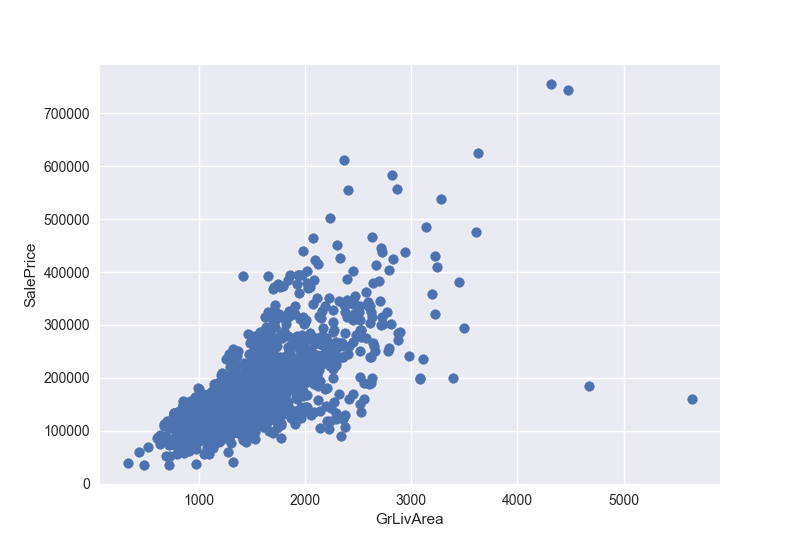
很明显看到另个异常值,我们先把这两个点删除

1
train = train.drop(train[(train['GrLivArea'] > 4000) & (train['SalePrice'] < 300000)].index)

目标变量

房价是我们需要预测的变量,所以我们先分析一下这个变量

1
2
3
4
5
6
7
8
9
10
11
12
13
14
15
16
sns.distplot(train['SalePrice'] , fit=norm)

# Get the fitted parameters used by the function
(mu, sigma) = norm.fit(train['SalePrice'])
print( '\n mu = {:.2f} and sigma = {:.2f}\n'.format(mu, sigma))

#Now plot the distribution
plt.legend(['Normal dist. ($\mu=$ {:.2f} and $\sigma=$ {:.2f} )'.format(mu, sigma)],
loc='best')
plt.ylabel('Frequency')
plt.title('SalePrice distribution')

#Get also the QQ-plot
fig = plt.figure()
res = stats.probplot(train['SalePrice'], plot=plt)
plt.show()

房价正态对比图以及QQ图

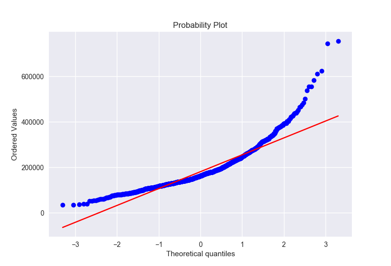
目标变量右偏,线性模型比较喜欢正态分布的数据,因此我们需要转换变量使其正态分布

对数据进行log变换

1
2
3
4
5
6
7
8
9
10
11
train['SalePrice'] = np.log(train['SalePrice'])
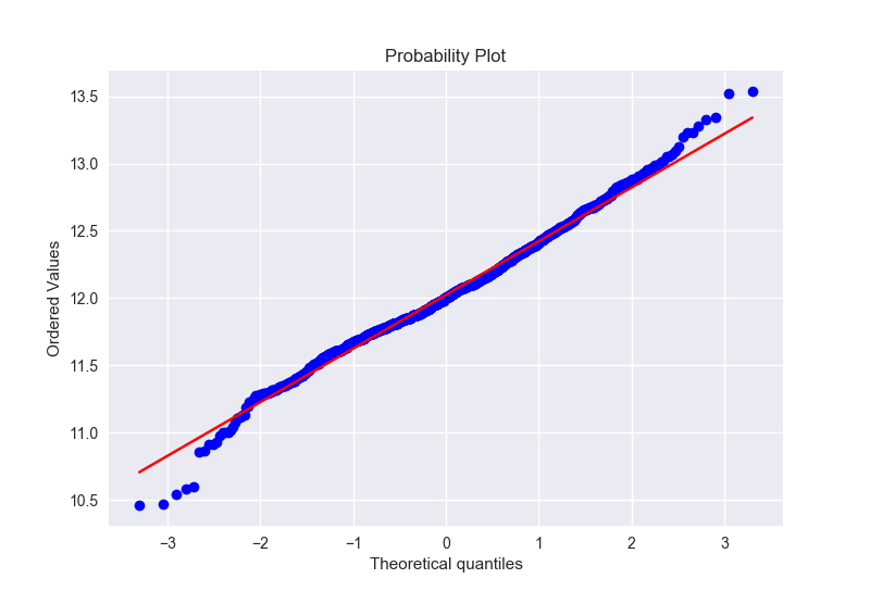
sns.distplot(train['SalePrice'],fit=norm)
(mu,sigma) = norm.fit(train['SalePrice'])
print('the $\mu$ = {:.2f} \n the $\sigma$ = {:.2f}'.format(mu,sigma))
plt.legend(['Norm distribution( $\mu$ = {:.2f} , $\sigma$ = {:.2f})'.format(mu,sigma)],loc='best')
plt.ylabel('Frequency')
plt.xlabel('SalePrice')
plt.title('SalePrice distribution')
fig = plt.figure()
stats.probplot(train['SalePrice'],plot=plt)
plt.show()

可以看到,变换之后更加接近正态分布

特征工程

先把所有train和test数据连接在一起,并删掉售价这列

1
2
3
4
5
6
all_data = pd.concat([train,test],ignore_index=True)
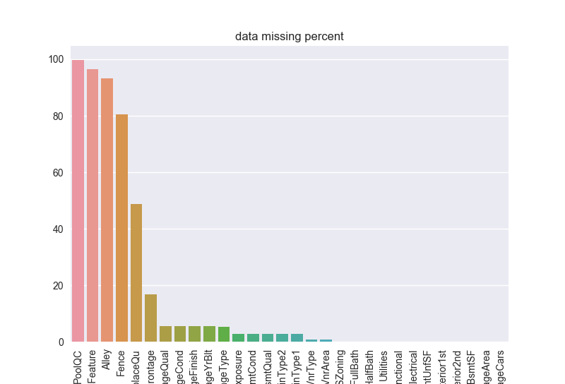
ntrain = train.shape[0]
ntest = test.shape[0]
y_train = train.SalePrice.values
all_data.drop('SalePrice',1,inplace=True)
print(all_data.shape)

缺失数据

先把缺失数据找出来

1
2
3
4
all_data_na = (all_data.isnull().sum() / len(all_data)) *100
all_data_na = all_data_na.drop(all_data_na[all_data_na == 0].index).sort_values(ascending=False)[:30]
missing_data = pd.DataFrame({'Missing Ratio':all_data_na})
print(missing_data.head(20))
Missing Ratio
PoolQC 99.691
MiscFeature 96.400
Alley 93.212
Fence 80.425
FireplaceQu 48.680
LotFrontage 16.661
GarageQual 5.451
GarageCond 5.451
GarageFinish 5.451
GarageYrBlt 5.451
GarageType 5.382
BsmtExposure 2.811
BsmtCond 2.811
BsmtQual 2.777
BsmtFinType2 2.743
BsmtFinType1 2.708
MasVnrType 0.823
MasVnrArea 0.788
MSZoning 0.137
BsmtFullBath 0.069

画一下缺失的比例:

1
2
3
4
sns.barplot(all_data_na.index,all_data_na.values)
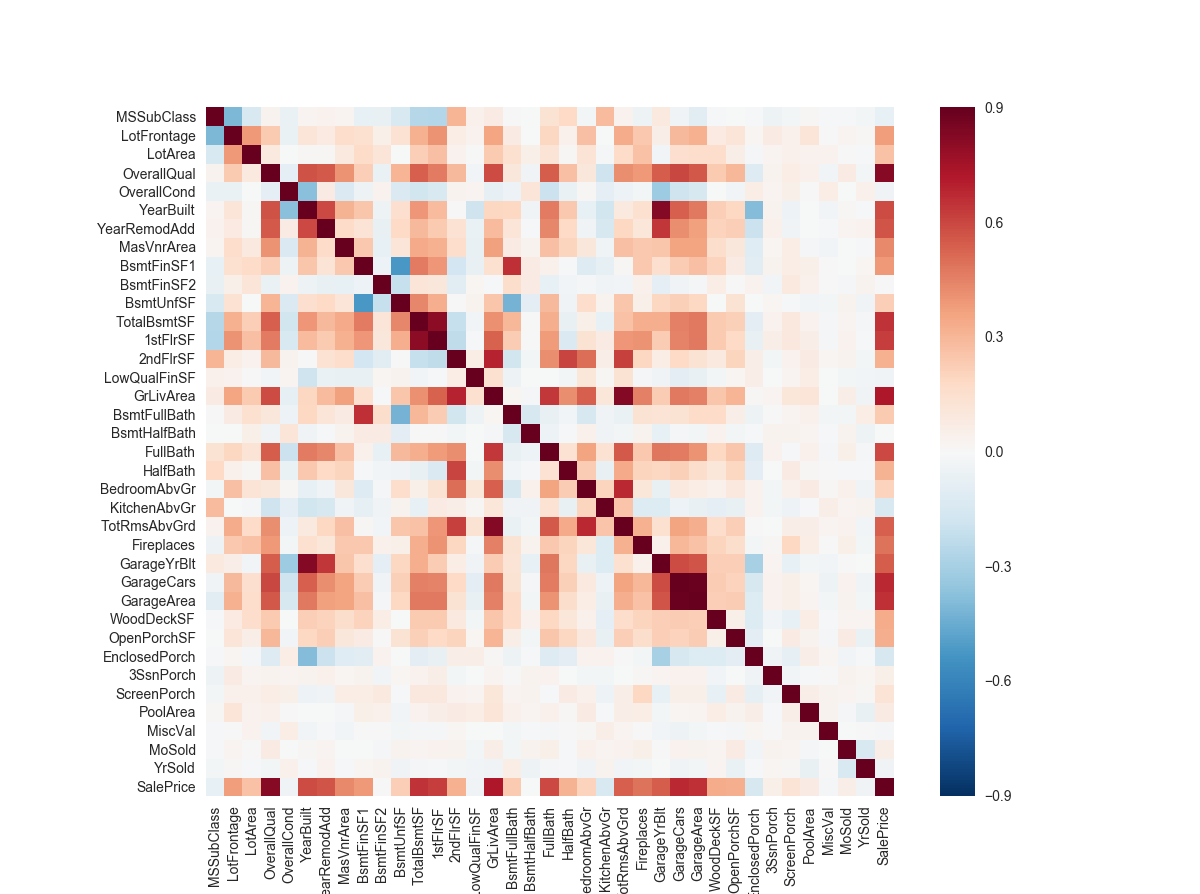
plt.xticks(rotation=90)
plt.title('data missing percent')
plt.show()

数据相关性分析

1
2
3
4
5
6
corrmat = train.corr()
plt.subplots(figsize=(12,9))
sns.heatmap(corrmat,vmax=0.9,square=True)
plt.xticks(rotation=90)
plt.yticks(rotation=360)
plt.show()

计算缺失值

  • PoolQC : 数据描述中提到 NA 表示 “No Pool”.

  • MiscFeature : 数据描述中提到 NA 表示 “no misc feature”

  • Alley : 数据描述中提到 NA 表示 “no alley access”

  • Fence : 数据描述中提到 NA 表示”no fence”

  • FireplaceQu : 数据描述中提到 NA 表示 “no fireplace”

  • ‘GarageType’, ‘GarageFinish’, ‘GarageQual’, ‘GarageCond’,’BsmtQual’, ‘BsmtCond’,’BsmtExposure’, ‘BsmtFinType1’, ‘BsmtFinType2’,’MSSubClass’: 用’None’替代缺失值

1
2
3
var = ['PoolQC','MiscFeature','Alley','Fence','FireplaceQu','GarageType', 'GarageFinish', 'GarageQual', 'GarageCond''MSSubClass']
all_data[var] = all_data[var].fillna('None')
print('为null的值',max(all_data[var].isnull().sum()))

LotFrontage: 由于连接到房产的每条街道的面积很可能与其附近的其他房屋具有相似的面积,因此我们可以通过邻里的LotFrontage填充缺失值。

1
all_data['LotFrontage'] = all_data.groupby('Neighborhood')['LotFrontage'].transform(lambda x: x.fillna(x.median()))
  • **’GarageYrBlt’, ‘GarageArea’, ‘GarageCars’,’BsmtFinSF1’, ‘BsmtFinSF2’, ‘BsmtUnfSF’, ‘TotalBsmtSF’,’BsmtFullBath’, ‘BsmtHalfBath’,’MasVnrArea’, ‘MasVnrType’**:用0代替缺失值
1
2
var = ['GarageYrBlt', 'GarageArea', 'GarageCars','BsmtFinSF1', 'BsmtFinSF2', 'BsmtUnfSF', 'TotalBsmtSF','BsmtFullBath', 'BsmtHalfBath','MasVnrArea', 'MasVnrType']
all_data[var] = all_data[var].fillna(0)
  • **’Electrical’,’MSZoning’,’KitchenQual’,’Exterior1st’,’Exterior2nd’,’SaleType’**:用它的频繁模式来填充缺失值
1
2
3
var = ['Electrical','MSZoning','KitchenQual','Exterior1st','Exterior2nd','SaleType']
for v in var:
all_data[v] = all_data[v].fillna(all_data[v].mode()[0])
  • Utilities : 这个变量在训练数据中,几乎所有值都是’AllPub’,除了两个NA和1个”NoSeWa”,所以我们可以删除这个变量。
1
all_data.drop('Utilities',1,inplace=True)
  • Functional : NA 表示 typical
1
all_data["Functional"] = all_data["Functional"].fillna("Typ")

再检查一下有没有缺失值:

1
print('缺失值个数:',max(all_data.isnull().sum()))
1
缺失值个数:0

更多的特征工程

将某些本来应该是类的数值变量变为类型变量

1
2
3
4
5
6
7
8
9
10
11
#MSSubClass=The building class
all_data['MSSubClass'] = all_data['MSSubClass'].apply(str)


#Changing OverallCond into a categorical variable
all_data['OverallCond'] = all_data['OverallCond'].astype(str)


#Year and month sold are transformed into categorical features.
all_data['YrSold'] = all_data['YrSold'].astype(str)
all_data['MoSold'] = all_data['MoSold'].astype(str)

然后将数值变量变成值:

1
2
3
4
5
6
7
8
columns = ('FireplaceQu', 'BsmtQual', 'BsmtCond', 'GarageQual', 'GarageCond',
'ExterQual', 'ExterCond','HeatingQC', 'PoolQC', 'KitchenQual', 'BsmtFinType1',
'BsmtFinType2', 'Functional', 'Fence', 'BsmtExposure', 'GarageFinish', 'LandSlope',
'LotShape', 'PavedDrive', 'Street', 'Alley', 'CentralAir', 'MSSubClass', 'OverallCond',
'YrSold', 'MoSold')
for column in columns:
lb_make = LabelEncoder()
all_data[column] = lb_make.fit_transform(all_data[column].values)

加入一个额外的特征

我们都知道房价和总面积息息相关,那么我们在加一个总面积的变量

1
2
# Adding total sqfootage feature 
all_data['TotalSF'] = all_data['TotalBsmtSF'] + all_data['1stFlrSF'] + all_data['2ndFlrSF']

计算数值特征的数据斜度

1
2
3
4
5
6
7
numeric_feats = all_data.dtypes[all_data.dtypes != "object"].index

# Check the skew of all numerical features
skewed_feats = all_data[numeric_feats].apply(lambda x: skew(x.dropna())).sort_values(ascending=False)
print("\nSkew in numerical features: \n")
skewness = pd.DataFrame({'Skew' :skewed_feats})
skewness.head(10)
1
Skew in numerical features: 
Skew
MiscVal 21.940
PoolArea 17.689
LotArea 13.109
LowQualFinSF 12.085
3SsnPorch 11.372
LandSlope 4.973
KitchenAbvGr 4.301
BsmtFinSF2 4.145
EnclosedPorch 4.002
ScreenPorch 3.945

符合正态分布的变量斜度应该基本为0,离0越远表示越不符合正态分布

对高斜度变量进行box-cox变换

box-cox变换的公式

1
2
y = ((1+x)**lmbda - 1) / lmbda  if lmbda != 0
log(1+x) if lmbda == 0

找出斜度大于0.75的值

1
2
skewness = skewness[abs(skewness) > 0.75]
print("There are {} skewed numerical features to Box Cox transform".format(skewness.shape[0]))

进行box-cox变换

1
2
3
4
5
6
7
8
# 进行box-cox变换
skewness = skewness[abs(skewness)>0.75]
print('斜度大于0.75的有{}个'.format(skewness.shape[0]))
print(len(skewed_feats))
from scipy.special import boxcox1p
lam = 0.15
for feat in skewed_feats.index:
all_data[feat] = boxcox1p(all_data[feat],lam)

得到哑变量

1
2
all_data = pd.get_dummies(all_data)
print(all_data.shape)

建立模型

首先导入一系列会用到的包

1
2
3
4
5
6
7
8
9
10
from sklearn.linear_model import ElasticNet, Lasso,  BayesianRidge, LassoLarsIC
from sklearn.ensemble import RandomForestRegressor, GradientBoostingRegressor
from sklearn.kernel_ridge import KernelRidge
from sklearn.pipeline import make_pipeline
from sklearn.preprocessing import RobustScaler
from sklearn.base import BaseEstimator, TransformerMixin, RegressorMixin, clone
from sklearn.model_selection import KFold, cross_val_score, train_test_split
from sklearn.metrics import mean_squared_error
import xgboost as xgb
import lightgbm as lgb

使用sklearn里面的cross_val_score函数进行交叉验证 ,但是这个函数没有乱序的功能,所以加了一行乱序到这个交叉验证过程中。

1
2
3
4
5
6
# 交叉验证
n_folds = 5
def rmsle_cv(model):
kf = KFold(n_folds, shuffle=True, random_state=42).get_n_splits(train.values)
rmse = np.sqrt(-cross_val_score(model, train.values, y_train, scoring='neg_mean_squared_error',cv=kf))
return rmse
  • 交叉验证:用相同的数据进行学习和测试,这是机器学习中常见的一种错误,因为这样会过拟合。这样的测试效果是100%正确,但当模型用于新的数据时,得到的结果往往非常差。因此,常常将数据分为训练集和测试集合。
    在scikit-learn中,为了将数据随机切分,我们可以依靠train_test_split函数,导入iris数据集进行测试

    1
    2
    3
    4
    5
    6
    7
    8
    9
    10
    11
    12
    13
    14
    15
    16
    17
    18
    19
    20
    21
    >>> import numpy as np
    >>> from sklearn.model_selection import train_test_split
    >>> from sklearn import datasets
    >>> from sklearn import svm

    >>> iris = datasets.load_iris()
    >>> iris.data.shape, iris.target.shape
    ((150, 4), (150,))

    # 随机分40%的数据为测试集
    >>> X_train, X_test, y_train, y_test = train_test_split(
    ... iris.data, iris.target, test_size=0.4, random_state=0)

    >>> X_train.shape, y_train.shape
    ((90, 4), (90,))
    >>> X_test.shape, y_test.shape
    ((60, 4), (60,))

    >>> clf = svm.SVC(kernel='linear', C=1).fit(X_train, y_train)
    >>> clf.score(X_test, y_test)
    0.96...

    在调整参数的时候,那些超参需要手动调节,比如SVM中的C,这样仍然存在过拟合的风险,因为你需要不断调整参数使估计量最优。为了解决这个问题,我们再保留一部分数据,称之为验证集。在训练集上训练,在验证集上调参,最终在测试集上进行测试。
    然而,这种办法将数据集分成了三部分:训练集,验证集和测试集,可以用于训练模型的数据就非常少了,并且结果很大程度上取决于三部分的划分方法。
    这个问题的解决办法就是交叉验证(CV),在交叉验证中,仍然需要测试集,但是不在需要验证集。交叉验证最基本的方法就是k-fold 交叉验证:

    • 训练集被分为k个小的集合;
    • 用k-1个folds的数据进行训练
    • 余下的一个folds数据被用于验证模型

    最终模型的性能就是k折交叉验证循环中的平均值。

  • 计算交叉验证矩阵
    最简单的方法就是cross_val_score函数

    1
    2
    3
    4
    5
    >>> from sklearn.model_selection import cross_val_score
    >>> clf = svm.SVC(kernel='linear', C=1)
    >>> scores = cross_val_score(clf, iris.data, iris.target, cv=5)
    >>> scores
    array([ 0.96..., 1. ..., 0.96..., 0.96..., 1. ])

    平均的模型精度的95%置信区间就是:

    1
    2
    >>> print("Accuracy: %0.2f (+/- %0.2f)" % (scores.mean(), scores.std() * 2))
    Accuracy: 0.98 (+/- 0.03)

    可以通过传入不同的score方法来返回不同的结果

    1
    2
    3
    4
    >>> from sklearn import metrics
    >>> scores = cross_val_score(clf, iris.data, iris.target, cv=5, scoring='f1_macro')
    >>> scores
    array([ 0.96..., 1. ..., 0.96..., 0.96..., 1. ])
  • score的类型可以查看The scoring parameter: defining model evaluation rules
    我们也可以传入打乱的cv

    1
    2
    3
    4
    5
    6
    >>> from sklearn.model_selection import ShuffleSplit
    >>> n_samples = iris.data.shape[0]
    >>> cv = ShuffleSplit(n_splits=3, test_size=0.3, random_state=0)
    >>> cross_val_score(clf, iris.data, iris.target, cv=cv)
    ...
    array([ 0.97..., 0.97..., 1. ])

基本模型的构建

这里采用了五个基本模型:LASSO Regression (拉索回归),Elastic Net Regression (弹性网络回归),Kernel Ridge Regression (内核岭回归),XGBoost,LightGBM

1
2
3
4
5
6
7
8
9
10
11
12
13
14
15
16
17
18
19
20
21
22
23
24
25
26
27
28
29
30
31
32
33
34
# 基本模型
# LASSO Regression :拉索回归,用RobustScaler做中间键增强模型稳定性
lasso = make_pipeline(RobustScaler(), Lasso(alpha =0.0005, random_state=1))

#Elastic Net Regression :弹性网络回归,用RobustScaler做中间键增强模型稳定性
ENet = make_pipeline(RobustScaler(), ElasticNet(alpha=0.0005, l1_ratio=.9, random_state=3))

# Kernel Ridge Regression :内核岭回归,以huber作为损失函数提高稳定性
KRR = GradientBoostingRegressor(n_estimators=3000, learning_rate=0.05,
max_depth=4, max_features='sqrt',
min_samples_leaf=15, min_samples_split=10,
loss='huber', random_state =5)

#Gradient Boosting Regression : :
GBoost = GradientBoostingRegressor(n_estimators=3000, learning_rate=0.05,
max_depth=4, max_features='sqrt',
min_samples_leaf=15, min_samples_split=10,
loss='huber', random_state =5)

#XGBoost :
model_xgb = xgb.XGBRegressor(colsample_bytree=0.4603, gamma=0.0468,
learning_rate=0.05, max_depth=3,
min_child_weight=1.7817, n_estimators=2200,
reg_alpha=0.4640, reg_lambda=0.8571,
subsample=0.5213, silent=1,
random_state =7, nthread = -1)

#LightGBM :
model_lgb = lgb.LGBMRegressor(objective='regression',num_leaves=5,
learning_rate=0.05, n_estimators=720,
max_bin = 55, bagging_fraction = 0.8,
bagging_freq = 5, feature_fraction = 0.2319,
feature_fraction_seed=9, bagging_seed=9,
min_data_in_leaf =6, min_sum_hessian_in_leaf = 11)

看看每个模型单独的效果:

1
2
3
4
5
6
7
8
9
10
11
12
score = rmsle_cv(lasso)
print("\nLasso score: {:.4f} ({:.4f})\n".format(score.mean(), score.std()))
score = rmsle_cv(ENet)
print("ElasticNet score: {:.4f} ({:.4f})\n".format(score.mean(), score.std()))
score = rmsle_cv(KRR)
print("Kernel Ridge score: {:.4f} ({:.4f})\n".format(score.mean(), score.std()))
score = rmsle_cv(GBoost)
print("Gradient Boosting score: {:.4f} ({:.4f})\n".format(score.mean(), score.std()))
score = rmsle_cv(model_xgb)
print("Xgboost score: {:.4f} ({:.4f})\n".format(score.mean(), score.std()))
score = rmsle_cv(model_lgb)
print("LGBM score: {:.4f} ({:.4f})\n" .format(score.mean(), score.std()))

结果如下

1
2
3
4
5
6
7
8
9
10
11
Lasso score: 0.1115 (0.0074)

ElasticNet score: 0.1116 (0.0074)

Kernel Ridge score: 0.1176 (0.0081)

Gradient Boosting score: 0.1176 (0.0081)

Xgboost score: 0.1151 (0.0069)

LGBM score: 0.1162 (0.0071)

模型堆叠

最简单的堆叠方法: 平均基础模型

我们写个新的类用于模型堆叠,顺便对代码进行重构

写自己的估计函数的方法:

  • 首先决定你想要建立的方法,可能是四种之一:Classifier, Clusterring, Regressor and Transformer,Classifier是用于分类,Clusterring用于聚类,Regressor 用于回归预测,transform用于数据变换(输入一个数据x,返回数据的变化,比如PCA);
  • 选好之后,需要去继承BaseEstimator ,并选择合适的类型继承( ClassifierMixin, RegressorMixin, ClusterMixin, TransformerMixin);
  • 然后重写,__init__方法,fit方法(返回self,即为模型的训练方法),以及predictscore方法
1
2
3
4
5
6
7
8
9
10
11
12
13
class AveragingModels(BaseEstimator, RegressorMixin, TransformerMixin):
def __init__(self, models):
self.models = models
def fit(self,X,y):
self.models_ = [clone(x) for x in self.models]

for model in self.models_:
model.fit(X,y)
return self

def predict(self,X):
predictions = np.column_stack([model.predict(X) for model in self.models_])
return np.mean(predictions, axis=1)

最后看看得到的结果:

1
2
3
averaged_models = AveragingModels(models = (ENet, GBoost, KRR, lasso))
score = rmsle_cv(averaged_models)
print(score.mean(),score.std())
1
0.1095002303790.00763453599777

复杂的融合方法:加入一个元模型

训练过程如下图:

  1. 将数据分成两部分,训练和保留部分
  2. 用训练数据训练多个基础模型
  3. 用保留部分的数据,测试基础模型
  4. 用第三步中得到的对保留部分数据的预测作为输入,加上正确的目标变量作为输出,去训练一个更高水平的模型,称为元模型

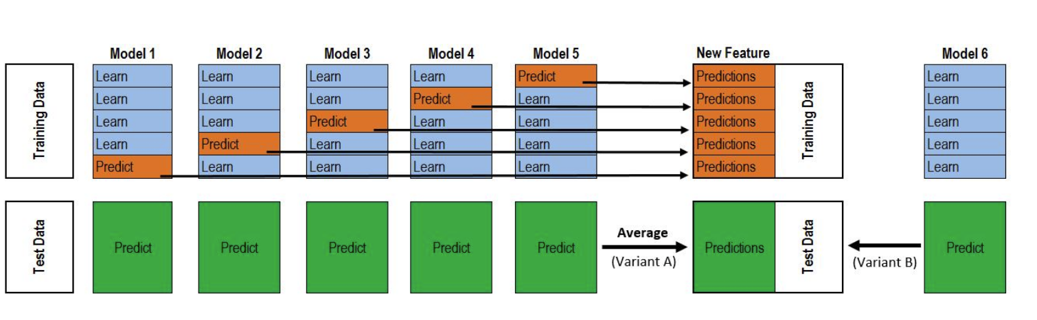
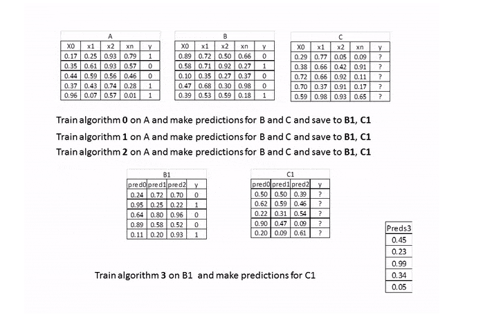
在上图中,A,B就是训练数据集,被分成了训练A和保留B,两部分。基础模型是算法0,1,2,元模型是算法3,B1是新的特征用于训练元模型3,C1是最终需要预测的元特征。

Stacking averaged Models Class

1
2
3
4
5
6
7
8
9
10
11
12
13
14
15
16
17
18
19
20
21
22
23
24
25
26
27
28
29
30
31
32
33
34
35
36
class StackingAveragedModels(BaseEstimator, RegressorMixin, TransformerMixin):
def __init__(self, base_models, meta_model, n_folds=5):
self.base_models = base_models
self.meta_model = meta_model
self.n_folds = n_folds

# We again fit the data on clones of the original models
def fit(self, X, y):
self.base_models_ = [[]] * len(self.base_models)
self.meta_model_ = clone(self.meta_model)
kfold = KFold(n_splits=self.n_folds, shuffle=True, random_state=156)
out_of_fold_predictions = np.zeros((X.shape[0], len(self.base_models)))

for i, model in enumerate(self.base_models):
for train_index, holdout_index in kfold.split(X, y):
#base_models_长度为模型的个数
#五折交叉之后,每种模型得到了五个可用的模型,都保存在base_models_[i]中
instance = clone(model)
self.base_models_[i].append(instance)
instance.fit(X[train_index], y[train_index])
y_pred = instance.predict(X[holdout_index])
out_of_fold_predictions[holdout_index, i] = y_pred
# 用的到的[原始数据行数*模型个数]的特征训练新的回归算法
self.meta_model_.fit(out_of_fold_predictions, y)
return self

# Do the predictions of all base models on the test data and use the averaged predictions as
# meta-features for the final prediction which is done by the meta-model
def predict(self, X):
# 每个模型预测X的结果作为特征输入,用心的预测算法预测出最终结果
meta_features = np.column_stack([np.column_stack([model.predict(X) for model in base_models]).mean(axis=1) for base_models in self.base_models_])
return self.meta_model_.predict(meta_features)

stacked_averaged_models = StackingAveragedModels(base_models = (ENet, GBoost,KRR,GBoost,model_xgb,model_lgb),meta_model = lasso)
score = rmsle_cv(stacked_averaged_models)
print("Stacking Averaged models score: {:.4f} ({:.4f})".format(score.mean(), score.std()))

最终成绩